Total Variation Denoising

Working with data is an important part of my day-to-day work. No matter if it’s speech, music, images, brain waves, or some other stream of data there’s plenty of it and there’s always some quality issue associated with working with the data. In this post I’m interested in providing an introduction to one technique which can be utilized to reduce the amount of noise present in some of these classes of signals.

Noise might seem abstract at first, but it’s relatively simple to quantify it. If the original signal, $x$, is known, then the noise, $n$, is any deviation in the observation, $y$, from the original signal.

$$y = x + n$$

Typically the deviation is measured via the squared error across all elements in a given signal:

$$\text{error} = ||x-y||^2_2 = \sum_i (x_i-y_i)^2$$

When only the noisy signal, $y$, is observed it is difficult to separate the noise from the signal. There is a wealth of literature on separating noise and many algorithms focus on identifying underlying repeating structures. The algorithm that this post focuses on is one which reduces the total variation over a given signal. One example of a signal with little variation is a step function:

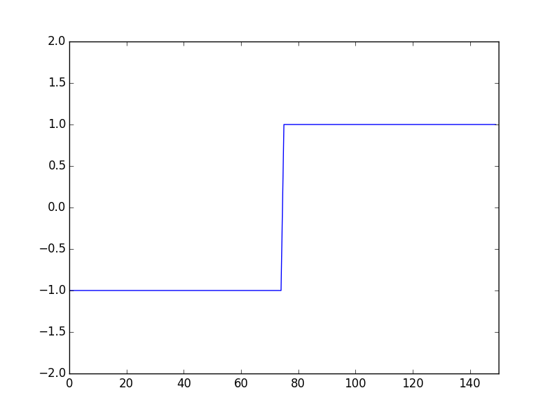
A step function only has one point where a sample of the signal varies from the previous sample. The Total Variation denoising technique focuses on minimizing the number of points where the signal varies and the amount the signal varies at each point. Restricting signal variation works as an effective denoiser as many types of noise (e.g. white noise) contain much more variation than the underlying signal. At a high level Total Variation (TV) denoising works by minimizing the cost of the output $y$ given input signal $x$ as described below:

$$\text{cost} = \text{error}(x, y) + \text{weight}*\text{sparseness}(\text{transform}(y))$$

Mathematically the full cost of TV denoising is:

$$ \begin{aligned} \text{cost} &= \text{error} + \text{TV-cost} \\ \text{cost} &= ||x-y||_2^2 + \lambda ||y||_{TV} \\ ||y||_{TV} &= \sum |y_i-y_{i-1}| \end{aligned}$$

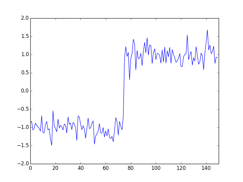
To see how the above optimization can recover a noisy signal, lets look at a noisy version of the step function:

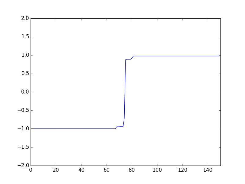
After using the TV norm to denoise only a few points of variation are left:

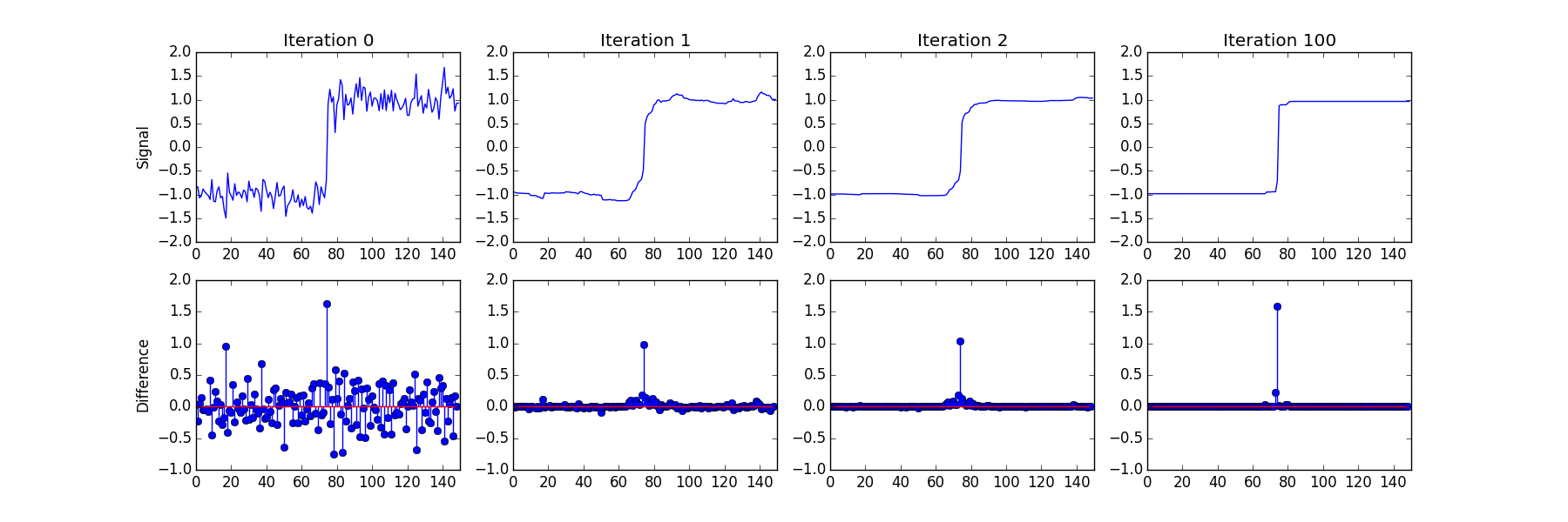
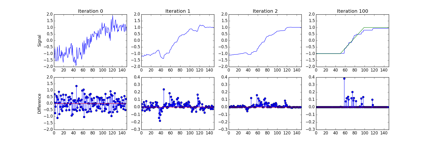
The process of getting the final TV denoised output involves many iterations of updating where variations occur. Over the course of iterations opposing variations cancel out and smaller variations are driven to $\Delta y = 0$. As the number of non-zero points increase a sparse solution is produced and noise is eliminated. For higher values of the TV weight, $\lambda$, the solution will be more sparse. For the noisy step function, $y$ and $\Delta y$ over several iterations look like:

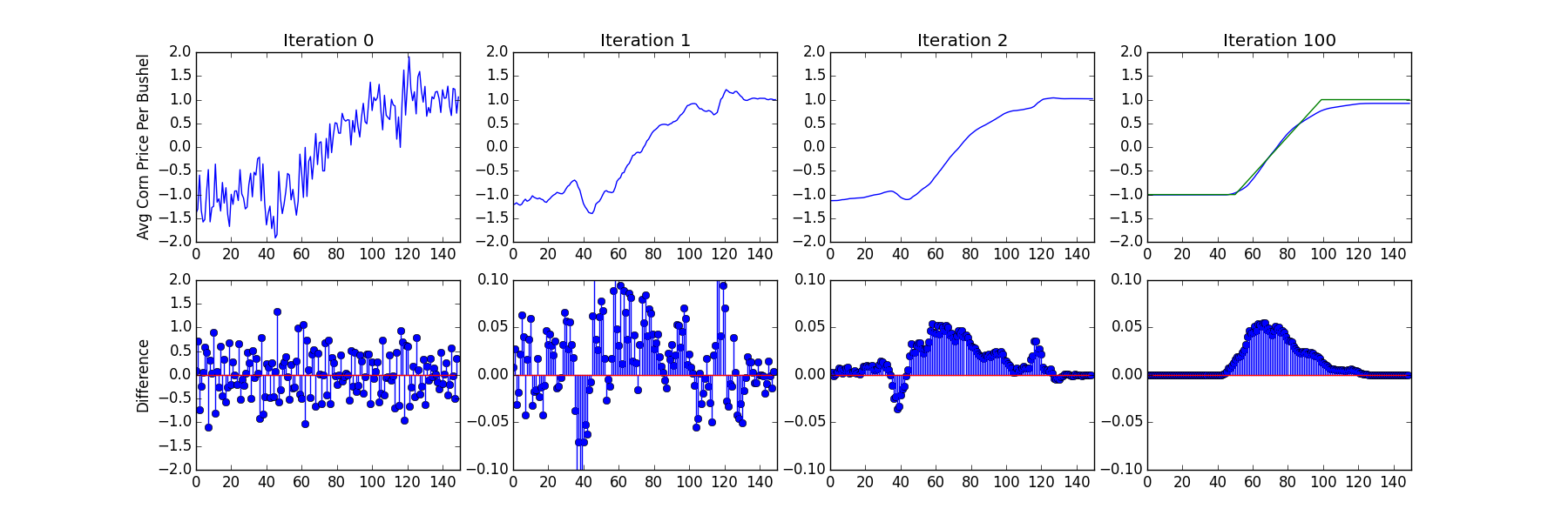
For piecewise constant signals, the TV norm alone works quite well, however there are problems which arise with the output when the original signal is not a series of flat steps. To illustrate this consider a piecewise linear signal. When TV denoising is applied a stair stepping effect is created as shown below:

One of the extensions to TV based denoising is to add 'group sparsity' to the cost of variation. Standard TV denoising results in a sparse set of points where there is non-zero variation, resulting in a few piecewise constant regions. With the TV norm, the cost of varying at point $\Delta y_i$ within the signal does not depend upon which other, $\Delta y_j,\Delta y_k,\text{etc}$, points vary. Group Sparse Total Variation, GSTV, on the other hand reduces the cost for smaller variation in nearby points. GSTV therefore generally produces smoother results with more gentle curves for higher order group sparsity values as variation occurs over several nearby points rather than a singular one. Applying GSTV to the previous example results in a much smoother representation which more accurately models the underlying data.

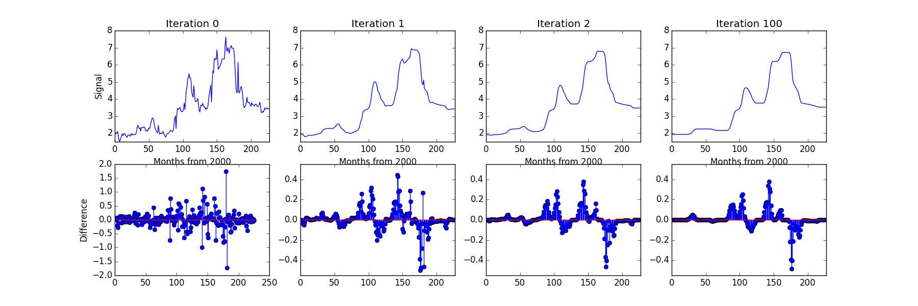
Now that some artificial examples have been investigated, lets take a brief look at some real world data. One example of data which is expected to have relatively few points of abrupt change is the price of goods. In this case we’re looking at the price of corn in the United States 2000 to 2017 in USD per bushel as retrieved from http://www.farmdoc.illinois.edu/manage/uspricehistory/USPrice.asp . With real data it’s harder to define noise (or what part of the signal is unwanted); However, by using higher levels of denoising the overall trends can be observed within the time-series data:

If this short into was interesting I’d recommend trying out TV/GSTV techniques on your own problems. For more in depth information there’s a good few papers out there on the topic with the original GSTV work being:

And if you’re using Julia, feel free to grab my re-implementation of Total Variation and Group Sparse Total Variation at https://github.com/fundamental/TotalVariation.jl